How Do You Fight Smog with Machine Learning? We Tried, and This Is What Happened


Carbon monoxide, nitrogen dioxide, particulates, and many other air pollutants form smog – the environmental nightmare hanging over cities in many countries. The smog levels in Poland frequently breach the statutory limits, especially in the winter, when the concentration of substances such as PM10 can exceed the norm by more than 500 percent. In 10Clouds, we decided to draw attention to the problem and motivate the local authorities to act immediately.
Our goal was to show the current pollution level for any place in Poland and be able to predict it for several hours ahead. It was a perfect opportunity for our team to work with machine learning. We used Python with a few additional libraries, which provided us with ready-made tools and models:
- Pandas
- Numpy
- Scikit-learn
- Keras
- xgboost
Python seemed like a good choice, because it offers a very wide selection of machine learning and data analysis tools, and it boasts a massive community we could always turn to in case we needed support.
Learning, teaching, studying
The first thing we needed was the data on the history of pollution levels, hourly pollution levels, and weather. A lot of data. We obtained it from the archives of the Chief Inspectorate of Environmental Protection (pollution levels) and the API of the Institute of Meteorology and Water Management (weather conditions).
The next step was to select a pollution measurement station and prepare the data for building the prediction model. We began with only one station, because to the geographical and weather conditions for each station vary, and it could potentially be problematic to generalize the model for many stations. We chose a station located at Marszałkowska Street, Warsaw, which measures the level of PM10, PM2.5, NO2, and CO.
Subsequently, we included time data such as the time of day and the day of the week, which are inherently cyclical. We wanted our model to be also based on factors such as increased traffic during the week, especially at peak hours, or a greater demand for heating in winter – they can both bump up pollution levels significantly.

The question we wanted to answer was: how can we make our machine learning model know that a feature is cyclical? In other words, we wanted our machine learning model to know that 23:59 and 00:01 are only 2 minutes apart, regardless of the day they fall on. The model only needed to know that some features are cyclical, and they would be similar for these hours – be it Monday or Thursday.
Firstly, we added a `sec` feature with the number of seconds from 01.01.1970. Then we created a variable `seconds_in_day` with the number of seconds in the day. The final trick was to transform one-time feature (i.e. time of the day) into two new features `sin_time` and `cos_time`. We can see it below, where `df` is a pandas data frame with all our data.
import numpy as np from datetime import datetime df['sec'] = [(datetime.strptime(i, '%Y-%m-%d %H:%M') - datetime(1970,1,1)).total_seconds() for i in df.index.values.tolist()] seconds_in_day = 24*60*60 df['sin_time'] = np.sin(2*np.pi*df.sec/seconds_in_day) df['cos_time'] = np.cos(2*np.pi*df.sec/seconds_in_day) Figure 1. shows exactly what we did. The distance comparisons between the points correspond to the difference in time. The same approach was used for other cyclic parameters (day of the week, day of the year etc.)
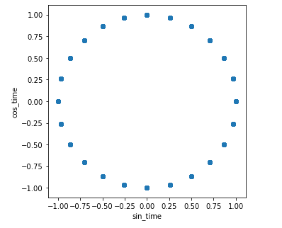
Figure 1. The relationship between the two introduced features
Unfortunately, we encountered several problems.
Houston, we have a (machine learning) problem
Take 1
The first problem was that if we wanted to predict the pollution values for several hours ahead, then we also needed to collect the weather values from the future or… predict them. This is due to the fact that our approach for long-term predictions was to calculate each next hour iteratively, using the vector from the previous hour.
In addition, air pollution measurement stations do not measure weather conditions, and the other way round – weather stations do not measure pollution levels. Even though the weather conditions were obtained as close as possible to the measurement station, those different locations caused a problem of mismatched conditions and weakened the correlation between weather and smog. Because of the above issues, we focused on predictions based only on pollutants and time features and put the issue of missing weather data from the future on hold.
The second problem was much more complicated because we had a significant number of unavailable data points (even one month length; see Figure 2) and we had to deal with it somehow.
Initially, we grouped the missing data points according to their lengths and we found out that most of them are very short (single hours). With that in mind, we tried to fill these single gaps with values predicted by the model, leaving only the longer periods unchanged.
Firstly, however, we had to choose one model to follow. We took the following steps:
- analyze the models’ performance based on the data with deleted rows with gaps
- select the best-performing model
- only later complete the missing values using a chosen model
At this point, we normalized all of our data by bringing the values to the range 0-1, and we were ready for the next phase – the prediction model.
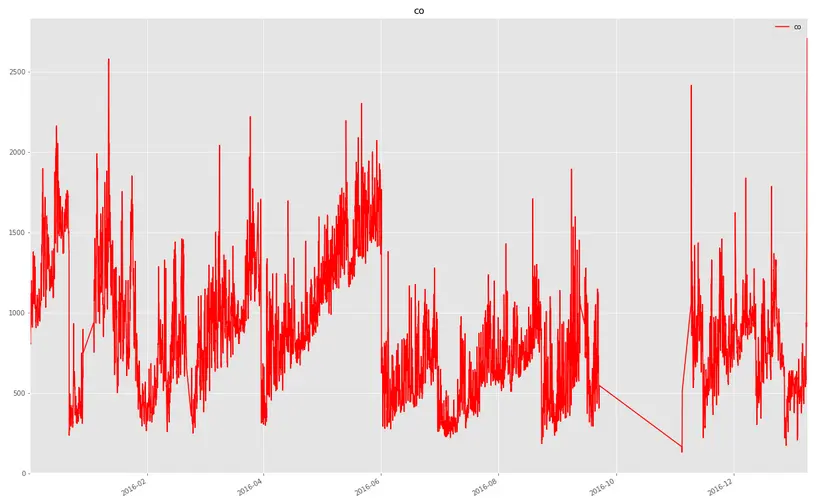
Figure 2. Carbon Dioxide values in 2016 for the Marszałkowska, Warsaw measurement station with the apparent lack of data between October and December
Considering the complexity of the subject, we decided that our goal will be to obtain accuracy that would be sufficiently high for the ordinary people. The main issue we needed to solve in our model was Time Series Predictions. The quality of our model was determined by the Root Mean Squared Error (RMSE). After the initial research phase, we chose three different approaches to start with:
- Classical Linear Regression
- Neural Networks
- XGBoost algorithm
Our input dataset was a simple matrix consisting of parameter values from singular hours and the output dataset was the vector with the values of the predicted parameter. We split our data into:
- a training dataset – 60% of the whole dataset – used to train models
- a validation dataset – 20% of the whole dataset – used to validate the performance of different models and fine-tune their parameters
- a test dataset – 20% of the whole dataset – used to evaluate the quality of the chosen model
We filed each machine learning model with the same data and tuned the parameters to obtain the best performance.
In Table 1, you can see the values of RMSE for the predictions for one hour ahead. As you can see, the XGBoost model gave the best results. The differences were not significant, but high enough to chose XGBoost to fill the missing values in our datasets.
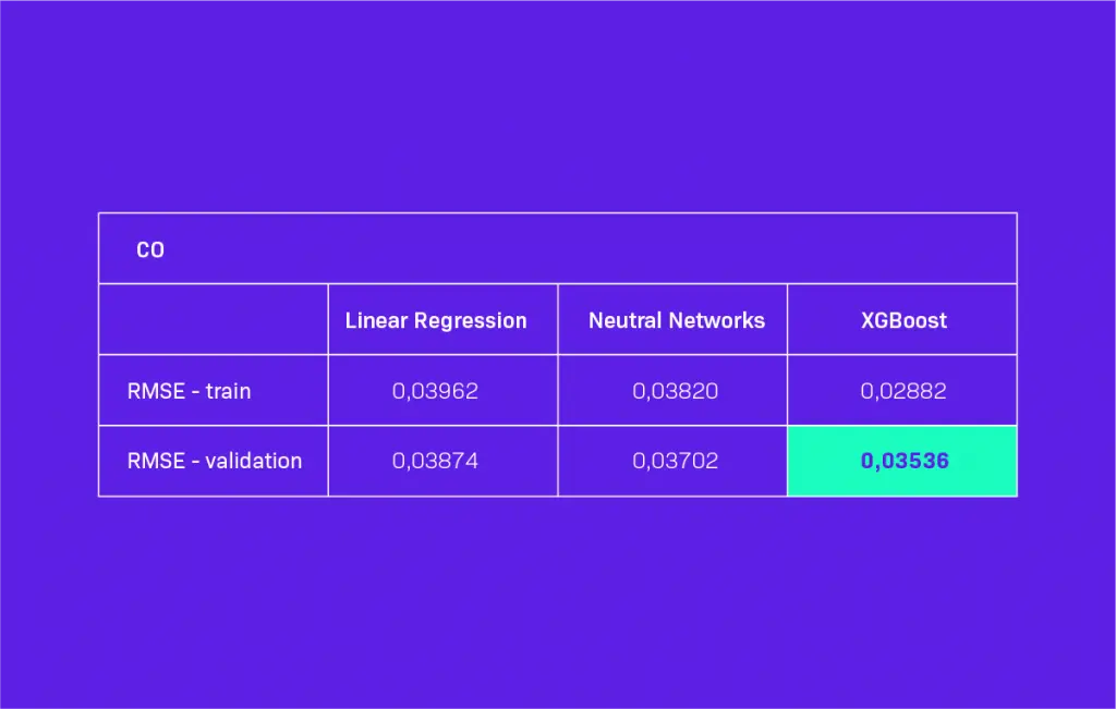
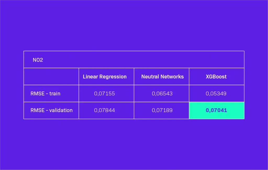
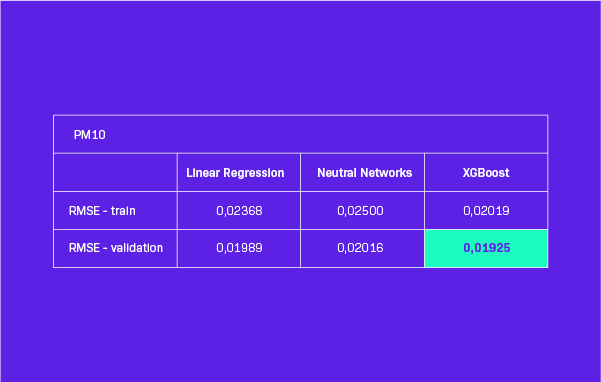
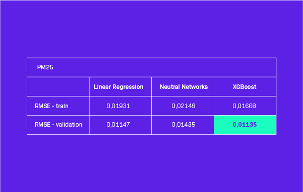
Table 1. Model Performance on dataset with gaps for 1 hour ahead predictions. Green color – best result.
Take 2
After predicting and filling the missing data, we decided to train our model once again using the newly obtained information. In Table 2, you can see the values of RMSE for the predictions for an hour ahead. This time we also checked the performance on the test dataset, not only on the validation dataset. As you can see, the XGBoost model again gave the best results in most cases.
However, in two cases (PM10 and PM25), the RMSE assumed significantly worse values for the XGBoost model. The differences were still not significant, but close enough for us to select XGBoost for further analysis. Nevertheless, we must keep in mind that XGBoost model did not perform best in all cases.
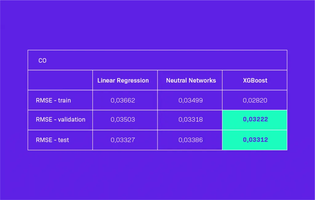
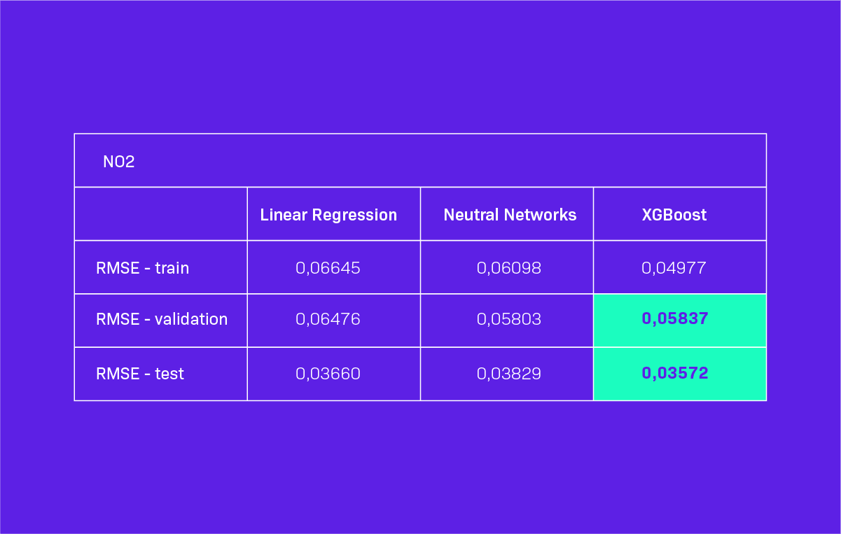

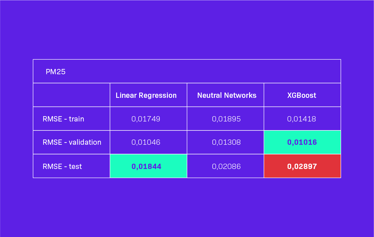
Table 2. Model Performance on consistent dataset for 1 hour ahead predictions. Green color = best result, red color = unexpected substantially worse RMSE values for the XGBoost model.
At this point, we needed to make one more choice, namely after completing the missing values, we could get many long vectors that consisted of parameter values from several consecutive hours. Keeping it in mind, we have developed 2 different approaches to teach our model.
The first approach, which we deemed ‘classic’, was identical to the approach used in choosing the model. In the other approach, which we called ‘vectors’, we prepared the input data differently. In the ‘vector’ approach, each row in the input matrix consisted of parameter values from several consecutive hours. We tried 4-, 6-, 8-, 12-, 24-, 48-hour vectors.
Figure 3 shows a chart with the values of RMSE for predictions for 24 hours ahead using the ‘classic’ approach, while Figure 4 presents the same figures for the ‘vectors’ approach. Long-term predictions were made iteratively by calculating the predictions for each next hour by using the vector from the previous hour (the ‘classic’ approach) or from n previous hours (the ‘vectors’ approach) as the input.
We thought that using data for more consecutive hours in the ‘vectors’ approach will enable our model to learn more about the conditions during a particular day, and we’ll get more precise predictions. We were rather surprised after comparing both approaches. To our surprise, we obtained only slightly better results with the ‘vector’ approach.
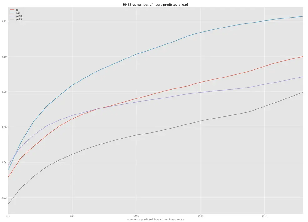
Figure 3. 24 hours predictions – ‘classic’ approach
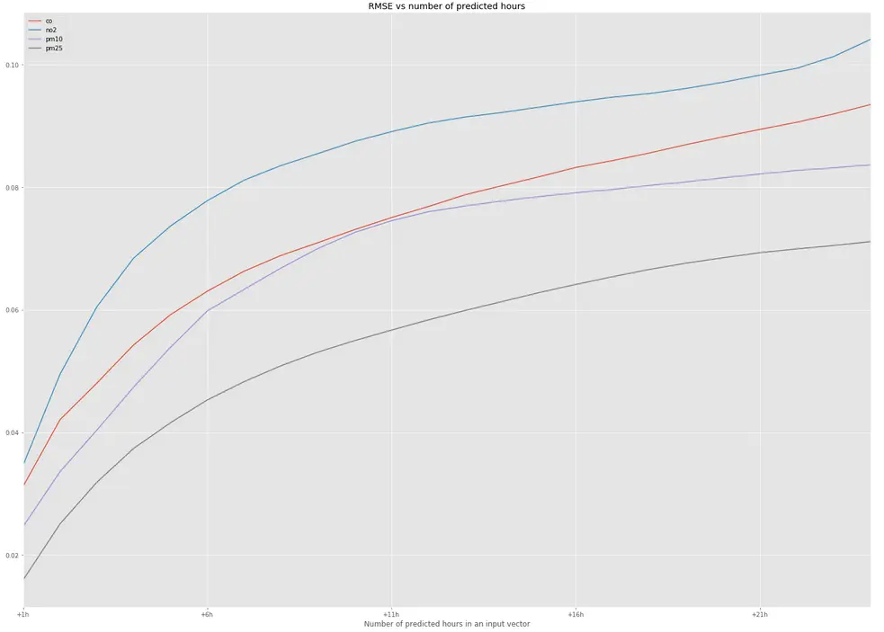
Figure 4. 24 hours predictions – ‘vector’ approach
Wrapping up
To sum up, we still have a lot of work to do. RMSEs that we obtained remain unsatisfactory. As you can see on the histograms in Figure 5, most PM10 and PM25 values are between 0.0 and 0.2. RMSE values between 0.01-0.03 for a prediction for one hour ahead seem promising, but for long-term predictions, the error grew considerably (i.e. 0.07-0.09 for 24 hours ahead).
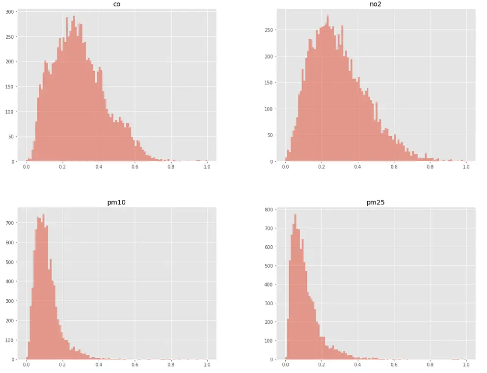
Figure 5. Value distribution for CO, NO2, PM10 and PM25
At this point, the predictions become too random. The situation is very similar for NO2 and CO levels. The next step for our team will be to improve the model’s performance in long-term forecasting, extend it to more stations and implement it in an application.
Apart from this internal project, we’ve already gathered experience with products utilizing machine learning, e.g. Trust Stamp. If you’re looking for developers to build your machine learning powered app, get in touch!
Resources
Chief Inspectorate of Environmental Protection in Poland
Encoding cyclical continuous features – 24-hour time by Ian London